The Beauty of Reinforcement Learning (2) - Reinforce with Baseline, A2C & GAE

Reducing the variance of policy gradient algorithms, from REINFORCE with baseline to A2C, to GAE that gracefully unifies them all.

In the last post, we contrasted reinforcement learning with classification problems, which helped us derive the Vanilla Policy Gradient (VPG) algorithm for optimizing policy using gradient. We also discussed the high variance problem with its gradient, which is given by

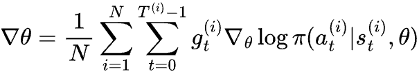
where g_t is the return starting from state s_t of an episode.

Investigating improvements to the algorithm to reduce variance is today’s topic.

REINFORCE with baseline

Let’s recall the sources of the high variance to find inspiration for a solution. Suppose that at state s_t, there are multiple actions the agent can choose from, all of which lead to a positive return g_t. Because g_t is always positive, no matter what action a_t is sampled, the gradient update will push θ to increase π(a_t|s_t; θ). This is bad because some actions might be worse than average, and therefore the gradient update can push θ to decrease expected return. The algorithm is still correct because when better actions get sampled, they will push θ harder (because of larger g_t) to other directions. However it does lead to high variance of gradient and thus unstable learning.

The thought experiment above suggests that what matters is not the absolute return following an action, but how much better or worse the return is than the average case under the current policy. If somehow we know the average return for every s_t, we can then use the difference between g_t and the average return to substitute for g_t in the formula above. With this change, if the return is better than average, the gradient will update θ to increase π(a_t|s_t; θ); otherwise the gradient will decrease π(a_t|s_t; θ), resulting in a stabler improvement trajectory.

The average returns from a state s is called its state value, denoted as v_π(s). It is formally defined as the expected return when the agent starts from state s, following π to take actions thereafter. The subscript π in the notation emphasizes that state values depend on the policy.

Now the question is, how can we calculate v_π(s) for all the states? By definition we can sample a lot of episodes to approximate, but this is intractable because a typical reinforcement learning problem has an astronomical number of states. Notice that g_t is a noisy sample of v_π(s), we could build a regression model v_π(s; w) to approximate state value, using g_t as the label. Since approximating state value is a regression problem, we can use mean square error loss to optimize its parameters. Every time we sample N episodes, we would use them to update both θ and w, namely,

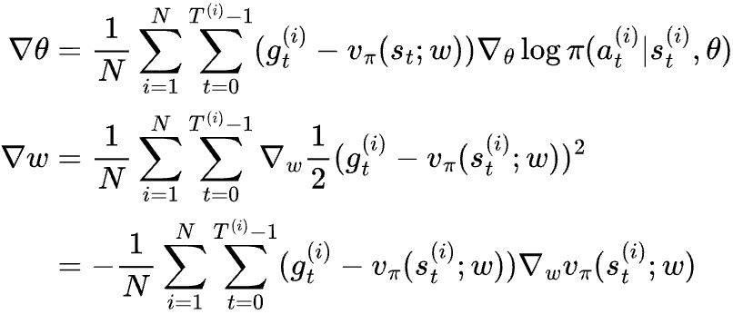
This revised algorithm is called “REINFORCE with baseline”. One interesting property of REINFORCE with baseline is that a bad estimate of v_π(s) affects the variance of the gradients, but it won’t create biases for the gradient, as in, the expectation of the gradient will still point towards maximizing expected return of an episode. This makes sense because subtracting a number that is the same for all actions of the same state doesn’t change the relative value of the actions; it only affects the likelihood of one sampled action generating gradient in the right direction.

Advantage Actor-Critic

REINFORCE with baseline addresses one source of variance but not all of them. g_t is a high variance random variable as it is the sum of multiple statistically correlated random variables (rewards). Because of its high variance, g_t - v_π(s_t) is still likely going to update the gradient in the wrong direction.

The problem stems from the fact that for an episode, we attribute g_t - v_π(s_t) solely to the choice of action a_t, while it is the outcome of a series of actions. If we sample lots of episodes that start with taking action a_t at state s_t, and average all g_t - v_π(s_t), we can confidently attribute it to a_t. However, with just one episode, it is overwhelmed by specific actions sampled down the road. Ideally, we should be able to decompose g_t - v_π(s_t) to all actions involved, such that each action only takes credit (or blame) on what they are responsible for. It turns out the same concept of state value is the key to the solution; we just need to use it more aggressively.

Let’s say we followed a stochastic policy π and sampled an episode with 3 actions. The state values for states in the episode are v_π(s₀) = 100, v_π(s₁) = 60, v_π(s₂) = 50 and v_π(s₃) = 0 (terminal state). The rewards for the actions are r₁ = 40, r₂ = 40, and r₃ = 40. Since the total return of the episode (i.e. g₀) is 120 but the average return for s₀ is 100, the question would be, which actions that got sampled should be credited for the difference of 20?

Looking at each step closely, we noticed:

• At s₀, taking action a₀ led to an immediate reward r₁=40. Since the state value of the next state v_π(s₁) = 60, we expect the return to be 40+60=100 by taking a₀, which is equal to the state value of s₀. This suggests that we didn’t get more reward than expected by taking action a₀, and we shouldn’t assign any credit to a₀.

• At s₁, taking action a₁ led to an immediate reward r₂=40. Since v_π(s₂) = 50, we expect the return to be 40+50=90 by taking a₁. Since 90-60=30, it means we got 30 more rewards than expected by taking a₁, and we should assign a credit of 30 to a₁.

• At s₂, taking action a₂ led to an immediate reward r₂=40. Since v_π(s₃) = 0, we expect the total future reward to be 0+40=40 by taking a₂, which is 10 less rewards than expected. We should therefore assign a credit of -10 to a₂.

Now, we have assigned credits to actions in the episode: 0 for a₀, 30 for a₁, -10 for a₂. They sum up to 20, exactly the amount that we need to credit to the actions.

More formally, the credit we assign for action a_t under state s_t is v_π(s_t+1) + r_t+1 - v_π(s_t). This term is called temporal difference error, or TD error. Using the same regression model v_π(s_t; w) to estimate v_π(s_t), we get an estimated TD error of v_π(s_t+1; w) + r_t+1 - v_π(s_t, w). Replacing g_t - v_π(s_t; w) with estimated TD error, we get:

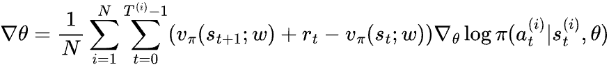
This algorithm is called Advantage Actor-Critic algorithm or A2C for short. Model π(a|s; θ) is called the actor because it predicts the stochastic actions to take. Model v_π(s; w) is called the critic as it is used to assess the “goodness” of the actions taken by the agent. The term v_π(s_t+1; w) + r_t+1 - v_π(s_t, w) estimates the advantage of a_t over other actions.

Compared to REINFORCE with baseline, A2C uses TD error that includes only one random variable r_t+1, which has much lower variance. It is independent of sampled rewards from future states and therefore, the coefficients of the gradients in its formula are much less correlated, contributing to a much smaller overall variance for ∇θ.

But not everything is good news. v_π(s_t+1; w) is a biased estimate of v_π(s_t+1), so the estimated advantage of action a_t, namely v_π(s_t+1; w) + r_t+1 - v_π(s_t; w) is biased as well as the overall gradient ∇θ. Contrasting REINFORCE with baseline, A2C introduces bias to the gradient, which will cause the algorithm’s failure to converge to a local maximum, even with large batches of episodes.

Generalized Advantage Estimator

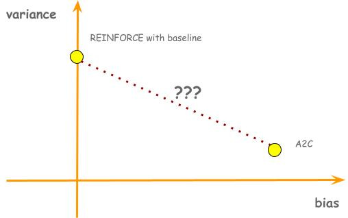
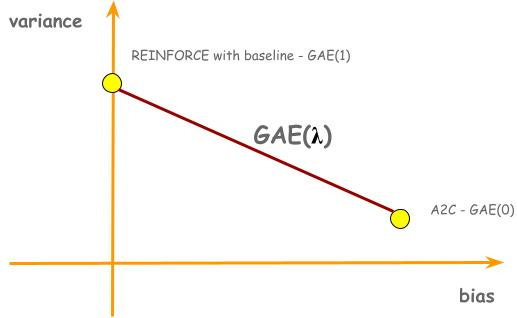
So far in this post we have discussed two policy gradient algorithms. Both of them use an estimated advantage of an action to decide how much to increase or decrease the probability of the action, but they exhibit trade-offs between bias and variance. REINFORCE with baseline estimates advantage using g_t - v_π(s_t; w); it has no bias, but high variance. A2C estimates advantage using v_π(s_t+1; w) + r_t+1 - v_π(s_t, w); it has bias, but low variance. These two algorithms present two points in a bias-variance trade-off plane. The natural question to ask would be, is there a line that connects these two dots? In other words, is there a generalized algorithm where REINFORCE with baseline and A2C are just special cases?

To find out the answer, we need to understand the connections between these two advantage estimators. In the example in the previous chapter, we have shown that g₀ - v_π(s₀) can be decomposed into TD errors of every actions in the episode:

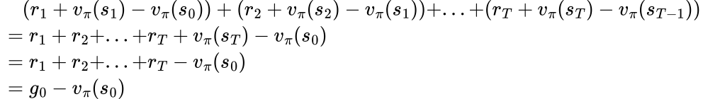
Apparently, this applies to all g_t - v_π(s_t):

So the connections between the two advantage estimators are clear: A2C only uses TD error of the next action, while REINFORCE with baseline sums up TD errors of all following actions. An obvious and somewhat naive way to generalize would be to estimate the advantage using the sum of TD errors of the next 2 actions, or 3 actions, etc. This is called N-step TD error but it has one caveat - why do we want to have a strict cutoff after N step?

Instead of doing a hard stop at N, a more graceful way is to use exponential decay. We will introduce a hyperparameter 𝛌 (0 ≤ 𝛌 ≤ 1) and multiply 𝛌^k to the k+1-th TD error. The new advantage estimator for action a_t becomes:

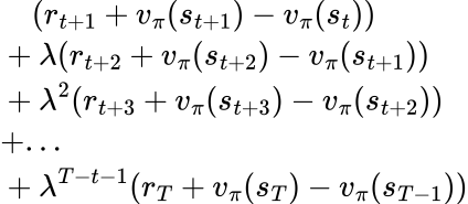
This is the Generalized Advantage Estimator or GAE for short. You can easily verify that when 𝛌=0, it becomes TD error, and when 𝛌=1, it becomes g_t - v_π(s_t). When 0<𝛌<1, we can see how bias is reduced compared to A2C. Suppose v_π(s_t+1) is overestimated by C, resulting in the first term of the advantage estimate to be overestimated by C. In A2C, a bias of C is what you get. In GAE though, the overestimate will be penalized by 𝛌C in the second term, reducing the bias from C to (1-𝛌)C.

Now, we have connected the dots:

GAE was introduced by John Schulman in 2015. Up until today, it is still a crucial component of state-of-the-art reinforcement learning algorithms.

What’s Next?

We have covered techniques to address the high variance problem of policy gradient algorithms. However, high variance is not the only problem.

Another problem is sample inefficiency. Vanilla Policy Gradient approaches policy optimization by asking the question of “what is the direction to update my policy based on what I can see”. Because of this framing, the sampled episodes can only be used for a small gradient step, and after that, they are discarded because the updated policy now sees a different world. State-of-the-art policy gradient methods like PPO (Proximal Policy Optimization), frame the policy improvement problem differently. Instead of just asking for direction to improve, PPO asks, “how can I make the biggest possible improvement to my policy based on what I can see?” It turns out that as long as the new policy stays not too far from the old one, we can keep using the outdated examples to update the new policy (with a slightly different objective), with some theoretical guarantee that the true objective will improve as well.