The Beauty of Reinforcement Learning (1) - Intro of Policy Based Methods

Reinforcement learning is powerful, beautiful and approachable - an intuitive yet in-depth introduction to reinforcement learning, including the what, why and how.

In the machine learning world, reinforcement learning is a mysterious creature. On one hand, it (or maybe she? he?) is very powerful. From dominating the Go game, to beating human world champions in playing Poker and Dota 2, to winning an IMO gold medal, it is the key to creating those magical AI moments. On the other hand, it appears to be quite unapproachable. Reinforcement learning problems and algorithms appear to be complex, requiring lots of tricks, tuning and compute resources to make them barely work. Most materials explaining them either involve lots of math and prior concepts, or are too high level for one to have a good understanding.

My goal with this series of posts is to demystify reinforcement learning, explaining it in-depth without involving deep math. Instead of focusing on the what, I want to focus on the why and how - the motivation behind the work, and how you can come up with the solution yourself through deep understanding of the problem, because I believe the why and how are the parts of learning with most endurable value. I also hope that through the deep understanding, you will find out that reinforcement learning is not just powerful, but also approachable, and beautiful.

Reinforcement Learning: Why and What

We are all familiar with classifiers - machine learning models that categorize data based on human labels. But the ultimate goal of machine learning is to build intelligent agents, which, driven by achieving their goal, can learn through continuously interacting with the environment and receiving feedback from the environment. Reinforcement learning aims to tackle this kind of problem.

Another reason why reinforcement learning is appealing is “the bitter lesson” articulated by the founder or modern reinforcement learning Richard Sutton. The bitter lesson points out that when enough compute resources are available, ML systems work better end to end without hard coded human prior knowledge. Lots of engineering work we do today, are all steps of achieving a bigger goal. If there is enough resource available, we might as well let the system learn end to end to achieve our goal - exactly the kind of problem that reinforcement learning is formulated for.

A reinforcement learning problem involves an agent and the environment which the agent is part of. Starting from an initial state of the environment s₀, the agent selects the next action a₀ to take, which leads to a reward r₁ and a new state s₁. The agent then takes another action a₁, leading to another reward r₂ and a new state s₂, so on and so forth, until the environment gets to a terminal state after T steps. This process generates a sequence of states, actions and rewards, which is called an “episode”. The cumulated reward in an episode is called the return. The rule that the agent follows, which can be stochastic, is called the “policy”, usually denoted as π. The goal of reinforcement learning is to find the optimal policy that maximizes the expected return.

An episode in reinforcement learning. The dotted lines are other possible states or actions that didn’t happen in this particular episode.

If we treat playing Go as a reinforcement learning problem, the state would be the positions of the stones and the initial state would be the empty board. The action of the agent is putting a stone at some position. The combination of the agent’s and the opponent’s move leads the game to the next state. The agent gets a reward of 0 for all the other states except for the terminal state, when they get a reward of 1 for a win, 0 for a tie and -1 for a loss.

Training LLM to solve math problems can also be considered a reinforcement learning problem. The sequence of tokens of a (random) question is the initial state. The LLM takes action by stochastically predicting the next token. Appending the predicted token to the sequence leads to the next state. The terminal state is when LLM outputs an EOS token. You can design the reward for the terminal state to be 1 for a correct final answer and 0 for a wrong final answer, but you can also add rewards for the format of the solution, such as conciseness, readability, etc. You may also give rewards to intermediate states for correct reasoning steps, similar to how a teacher scores a student’s work.

Vanilla Policy Gradient (REINFORCE)

There are many reinforcement learning algorithms and many ways to slice and dice them. In this series of posts, I will focus one important category of algorithms called policy based methods in which the agent directly learns what actions to take under a given state. RL algorithms used in today’s LLM post training such as PPO falls into this category.

In policy based methods, we model the policy π with parameters θ, which assigns a probability to an action given the current state s, denoted as π(a|s; θ). The idea is to start from an inferior initial policy (for example, one that takes random actions) and to iteratively update θ such that the model gives a higher and higher probability to actions that maximize the expected reward.

Similar to sampling random labeled examples in supervised learning, we would randomly sample a set of episodes. First, we randomly select a legitimate initial state, follow some stochastic policy to select an action to take, which leads to some reward and a future state. This keeps going until we reach the terminal state. Because we want to use gradients to improve the current policy, we should sample using the policy that we want to improve upon.

Because we want to sample random episodes to explore different actions, our initial policy has to be stochastic.

An episode with T steps are secretly T labeled examples

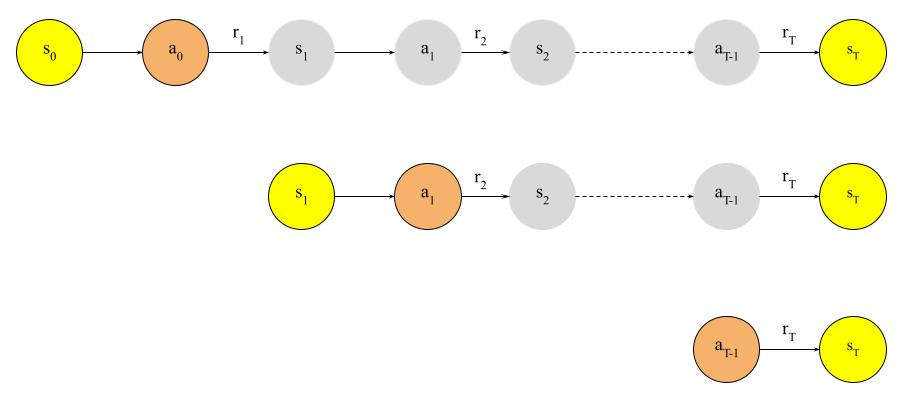
Let’s consider one sampled episode, which is a sequence of states, actions and rewards, s₀, a₀, r₁, s₁, a₁, r₂, …, r_T, s_T. Looking more closely, we can see that the model makes T predictions when we generate this episode:

• At s₀, the probability of taking action a₀ is π(a₀|s₀; θ). Taking action a₀ leads to a return of g₀ = r₁ + r₂ + … + r_T.

• At s₁, the probability of taking action a₁ is π(a₁|s₁; θ). Taking action a₀ leads to a return of g₁ = r₂ + r₃ + … + r_T.

• …

• At s_T-1, the probability of taking action a_T-1 is π(a_T-1|s_T-1; θ). Taking action a_T-1 leads to a return of g_T-1 = r_T.

If we think of a state as an example, the action as the label that we want to predict, the return would be the example weight that represents the importance of predicting the label correctly. In other words, an episode with T sequential actions are T labeled examples in disguise!

For classification problems, we maximize the (example weighted) accuracy of model f by maximizing the likelihood of predicting all the correct labels, i.e.

Using sum of log probabilities is a trick for numerical stability

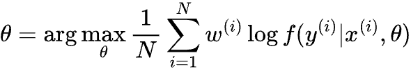
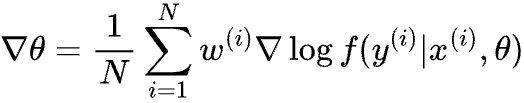
Where x⁽ⁱ⁾ is the feature of the i-th example, y⁽ⁱ⁾ is the label and w⁽ⁱ⁾ is the example weight. We then calculate the gradient of the maximization objective above, and update θ with learning rate ɑ:

Update θ by taking a step size of ɑ in the direction of its gradient

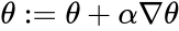
And we keep calculating the gradient and updating θ until some fixed number of steps, or the objective stops improving.

Similarly, to improve the policy, we can maximize the expected reward by maximizing “reward weighted” accuracy of predicting the actions. Replacing one classification example with T examples in an episode, we get

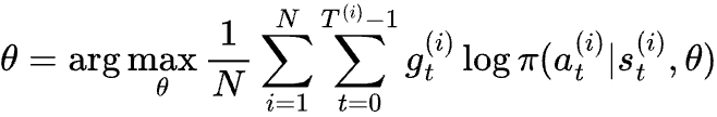
The gradient to update θ would be:

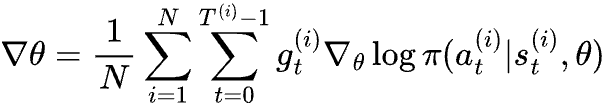
So, it looks like all we need to do for optimizing policy is sampling a batch of episodes, calculating the return for all the actions, and treating each action as an example (weighted by its reward) for classification. Pretty straight forward, right?

Well, not so fast.

Here comes one of the biggest differences between classification and reinforcement learning. For a classification problem, the labels and the weights won’t change as you update the model. However, this is not the case for reinforcement learning - the episodes are sampled according to your current policy, which will change once you update the parameters. When we encounter the same state, an updated policy is going to have a different probability distribution for taking different subsequent actions, leading to different expected returns. Therefore, a valid next update of θ will need to be based on a fresh sample from the updated policy.

Putting everything together, we get the following algorithm:

STEP 0: randomly initialize θ to get an initial stochastic policy π;

STEP 1: sample a batch of N episodes according to π;

STEP 2: calculate return gt for every state action pair, compute gradients and update θ;

STEP 3: if we reach a certain number of iterations, exit; otherwise, go back to STEP 1.

This is the simplest form of policy based methods, which is called Vanilla Policy Gradient (VPG for short), or REINFORCE after the 1993 paper that introduced the algorithm. For mathematical derivation of the algorithm, one can refer to OpenAI’s educational resource on reinforcement learning.

High Variance Problem with Vanilla Policy Gradient

VPG is a simple and elegant algorithm but it suffers from a couple of problems that make it inadequate for complex reinforcement learning problems. Today, we will just focus on one of them, which is high variance of the gradient of the optimization objective. In other words,

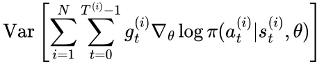
is high, compared to some other reinforcement learning algorithms. High variance of gradient causes parameters to be updated in a very unpredictable way, resulting in unstable learning. To combat high variance of VPG, one would need to sample large batches of episodes, and/or decrease the learning rate, which severely degrades sample efficiency.

To understand the source of high variance, we can compare VPG with classification. In fact, we can formulate a binary classification problem as a special one-step reinforcement learning problem. When the classifier predicts the right label, it gets a reward of a positive number w, and when it predicts the wrong label, it gets a reward of zero.

Classification is a special one-step reinforcement learning problem

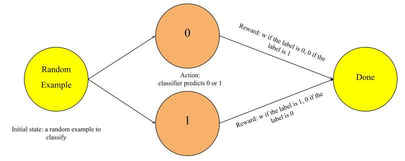
In this classification-as-reinforcement-learning problem, when the classifier makes a prediction and gets a return of w, we know that it is good because the opposite prediction will lead to a reward of 0. Because there is a unified baseline of zero return across all states, with the right set of features and clean labels, all the non-zero returns will push the model parameter in the same direction - increasing the probability of predicting the correct labels.

This is not the case for reinforcement learning in general. If action a_t at state s_t generates a return g_t of 0.5, is it a good action or not? It is hard to say. It is a good action if other actions generate a lower return, or a bad action if other actions generate a higher return. In other words, there is no unified baseline for returns across all states. With VPG, if a good action is sampled, it will push the gradient to one direction by some variable amount. If a bad action is sampled, it will push the gradient in some other direction by some other variable amount. The final outcome is the net effect of the two, which needs lots of examples to stabilize.

No unified baseline for returns across all states is one source of high variance, but not the only source. To make the analysis simpler, let’s ignore the gradient in formula (3), and just focus on the coefficient g_t. g_t is the sum of multiple random variables r_t+1, r_t+2, …, r_T and these random variables can be highly correlated. Furthermore, a reward r_t contributes to multiple returns - g₀, g₁, …, g_t-1 - which means all the coefficients are statistically correlated as well. Correlation is a serious problem. As an illustration, the variance of the number of heads of N independent coin flips is at most N/4, but if all the coin flips are correlated, the variance is N²/4 in the worst case. Correlation of g₀, g₁, …, g_T-1 causes the overall gradient to sway in unpredictable ways. The longer the episodes are, the higher variance there is.

The Credit Assignment Problem

The two sources of variance - no unified baseline across states, and variance and correlation of future returns in an episode - are fundamentally a credit assignment problem. When we seek ways to improve on top of the current policy, we shouldn’t look at the absolute returns. Instead, we should ask, is the return of this episode more or less than what is expected based on the current policy? Where does the gain or loss come from? What actions that the agent took in the episode should be credited for the gain or loss?

If we can identify the gain or loss of return compared to the expectation of the current policy, and credit the gain or loss to the right action, we have eliminated the noise and will be able to push the gradients in consistent directions.

In the next post of this series, I will talk about a couple of algorithms that addresses this credit assignment problem, with a trade-off between bias and variance.