The Beauty of Reinforcement Learning (3) - PPO Demystified

Including analogies that give you a vivid idea of how PPO works, and all the maths that you need to know PPO and its history thoroughly, end to end.

Credit: pexels.com

Imagine you are climbing a mountain on a dark and foggy night, so dark and foggy that even when you turn on your headlight, the only area that you can see clearly is the part right under your feet. You want to get to the top as fast as possible, but you also don’t want to take a reckless step and fall off the cliff. Here is the strategy you adopt. You examine the area under your foot, pick the steepest upward direction, but only take a tiny step forward in that direction to avoid stepping into an unpredictable area. After taking the step, you examine the area under your foot again before deciding your next step.

The progress will be slow but it seems to work. Well, except for two problems. For one, since you are only looking at the area right under your foot, you don’t know how big a step is safe. You might be right next to a cliff and therefore even a small step can take you off the cliff. Secondly, you know if you run out of battery for your headlight, you will be doomed. Battery is precious so you‘d rather turn the headlight off when you don’t need it. However, since you need to keep checking for every tiny step, there is no way to save battery.

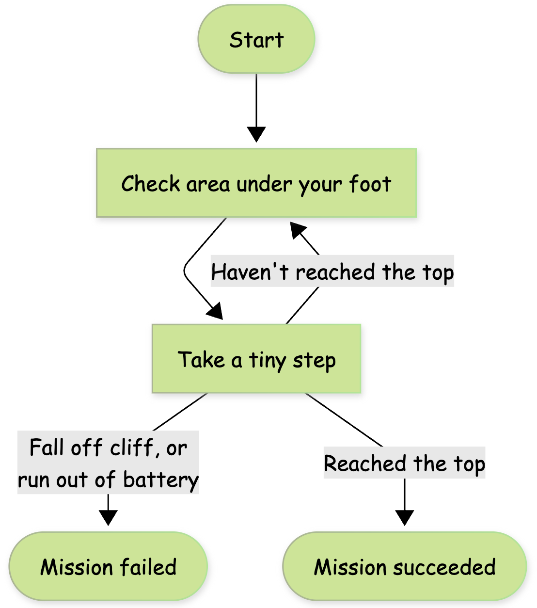
The mountain-climbing strategy above is the strategy of policy gradient methods we have discussed so far (REINFORCE, A2C, etc). They collect episodes based on the current policy (ML model that decides the agent's actions), estimate the gradient of the policy, and take a little step before collecting new examples based on the updated policy. However, because of the non-linearity of the policy model, a small step in terms of policy parameters can result in a drastic change of the policy, causing the whole upward learning trajectory to tank. More importantly, since the new policy is drastically different, it is very unlikely to collect new episodes that are similar to those sampled before, which means it is very hard to recover from the tanked learning trajectory.

The other problem with these algorithms is sample inefficiency. Sampling episodes require running the policy model and getting rewards from simulation or real environment, which can be expensive. However, these algorithms in principle can only use them once.

Fundamentally, A2C and algorithms alike only see one point in the mountain of policies, instead of a region. When the agent steps out of that point (which it always will) there is no guarantee what applies to the old point applies to the new one.

The PPO Strategy

So in order to save battery, and avoid missteps, you decide to take a different strategy that utilizes your skills. Instead of always keeping your headlight on, you turn the headlight on only when you are examining your surroundings. You use what you saw in your vague vision to build a mental map of your surroundings. You will then turn the headlight off and take multiple steps forward, before turning the headlight back on. The mental map gives you a direction (though an imperfect one) to aim for, such that you don't lose your direction when you step away from where you were. When you are too far away from your original place such that your mental map doesn't provide useful directions anymore, you turn your headlight back on to examine your surroundings again. You have greatly reduced the number of times you check your surroundings and your mental map gives you near term direction such that you can safely step out of the current spot. You are confident that you can safely get to the peak of the mountain.

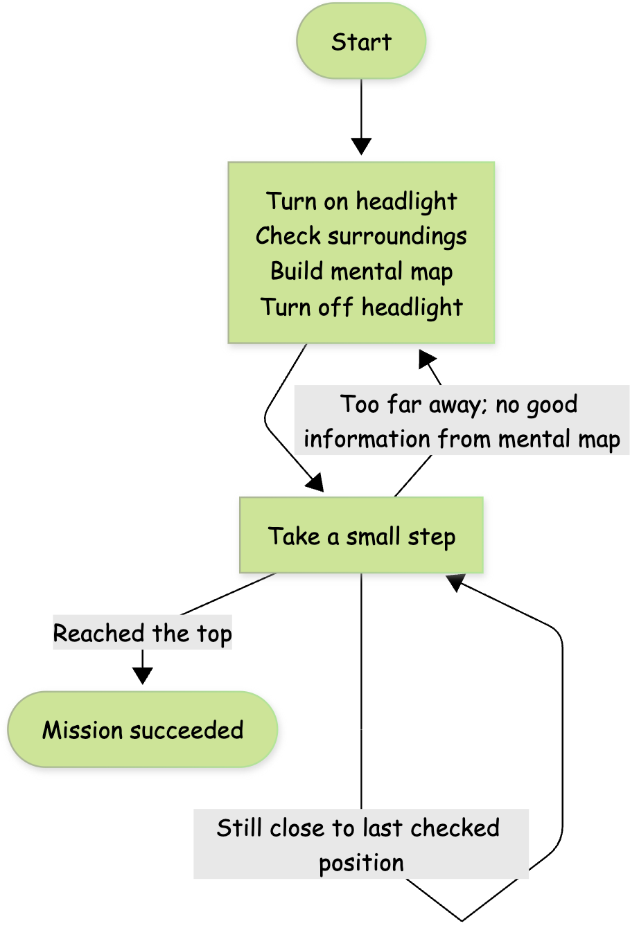
Your second strategy is the optimization strategy of Proximal Policy Optimization, or PPO for short, which updates the gradient multiple times using the same batch of episodes while trying to stay close to the current policy. More specifically it builds a cautious approximation of the nearby policies. You can safely derive gradients to update your policy based on the approximation, until you are getting too far away from the old policy. At that point, the cautious approximation contains no more useful information, and that’s when you resample episodes.

The strategy makes lots of sense, but there are a few technical questions to answer. How can we build a cautious approximation of the nearby policies and how do we know if it is a good approximation? How can we strike a balance between being cautious such that the agent doesn’t make unpredictable policy changes and being informative such that the agent can still make progress?

We will cover these questions below, but before that, let’s recap some essential concepts from the last two posts to set us up for deeper discussions.

State Value, Action Value and Advantage Function

In this post and my previous posts, I have been ignoring basic concepts like discounted reward. Including them won’t change any theories and conclusions presented here; I am omitting them for simpler math notation and explanation.

We talked a lot about advantage of an action in our last post, but let’s define it more formally this time. Let’s say at state s, if the agent follows policy π, it will get an expected future return of V_π(s). This is the state value of s. If at state s, instead of following policy π’s distribution to pick an action, the agent always takes action a, and follows π for future actions, the expected future return we get this way is called action value, denoted as Q_π(s, a). By definition, action value Q_π(s, a) is the expected reward the agent gets from taking action a, plus the state value of the next state the agent lands on, namely

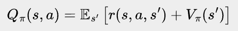
where r(s, a, s’) is the reward the agent gets by taking action a at state s and landing on s’. Note that in a stochastic environment, an action may land on different states with different probabilities. These probabilities are inherent to the environment and will not change due to the agent's action.

The advantage function of action a at state s under policy π is the difference between action value Q_π(s, a) and state value V_π(s), i.e.,

In other words, the advantage of an action at a certain state measures how much return we will gain or lose by forcing the agent to take that action instead of following the distribution of the policy. As we covered in the last post, future return minus state value, TD error, and GAE, are all ways to estimate the advantage function, with tradeoff between variance and bias.

One property of Advantage function will come in handy later:

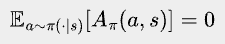
Here, a~π(·|s) means sampling an action a according to π’s probability distribution of actions at state s. The equation is actually quite obvious - some actions will be better than the state’s average, while others will be worse, but on average, the difference with the state's average is zero.

Learning from Slightly Off-Policy Examples

When we try to do multiple gradient updates with the same batch of episodes, the examples become “off-policy” after the first policy update, and therefore we need a way to learn from slightly off-policy data.

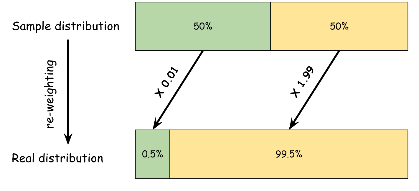
This problem is not unique to reinforcement learning; we deal with such problems in classification problems as well. Sometimes a class of interest is so rare that randomly collecting examples won’t give us enough positive labels. What we can do is stratified sampling - using some heuristic to oversample positive examples from a region where we know positive examples are more common. Now we have enough positive examples but the distribution of collected examples no longer reflects the real distribution. So in order to reflect the real distribution, we assign a weight to each example by how much they are downsampled or upsampled. In this way, our classifier’s scores can reflect the probability in the real distribution.

As we will see, re-weighting is the key to solving the off-policy example here as well. But first, we need to set up the formula where re-weighting can be applied.

One thing we learned from last post, is that for an arbitrary episode s₀, a₀, r₁, s₁, a₁, r₂, …, r_T, s_T, its return can be written as the state value of the initial state, plus the sum of TD errors:

Note that the π in the equation doesn’t need to be the policy that generates the episode; it can be any policy. Now, let’s suppose the episode is sampled from another policy π’. The expected return of π’, which we will denote as J(π’), is:

where E_π’[X] means the expectation of X over episode s₀, a₀, r₁, s₁, a₁, r₂, …, r_T, s_T, sampled following policy π’.

Let’s look at the first term E_π’[v_π(s₀)]. v_π(s₀) only depends on s₀, and thus E_π’[v_π(s₀)] equals J(π), which is the expected return of π.

Combining them together, we have

We like this formula because if you think of π’ as the policy that we are updating and π as the old policy that was used to sample the episodes, it expresses the change of return in terms of the old policy’s advantage functions.

Because of how we interpret π and π’, from here on, let’s change notation a bit. We will use π_old to replace π in the formula above, and use π to represent the policy that we are updating. Maximizing the new policy’s return thus becomes

The only problem with this maximization objective is that we cannot sample from π, as it is the policy we haven’t created yet. Directly optimizing it seems impossible; let's see if we can do some approximation.

The most forward way to approximate is to sample from the π_old instead of π, namely, we optimize

Instead. This is actually the learning objective of A2C, which gets back to where we were. We need a better approximation.

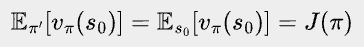
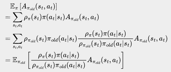
Take a closer look at E_π’[A_π(s_t, a_t)], the only parts of π’ that matter to the expectation are the probability of s_t at step t, and the probability of a_t given s_t. Let’s denote the probability of landing at s_t at step t when following policy π as ⍴_π(s_t). Now we can leverage the ratio between the two probability distributions to reweight a state action pair and map an expectation over the new policy to an expectation over the old policy.

What an achievement! Let’s take a break to celebrate.

Okay, back to work.

Now the expectation is based on the old policy π, which we can sample from, but since ⍴_π’(s_t) and ⍴_π(s_t) are hard to estimate, we still need some approximation. If we make a very rough approximation that ⍴_π’(s_t)π’(a_t|s_t) = ⍴_π(s_t)π(a_t|s_t), we go back to the objective of A2C again. However, we can make a weaker assumption that ⍴_π’(s_t)≅⍴_π(s_t), i.e. the state distribution at step t stays roughly the same between the new and old policies. This approximation makes sense when the policies are only slightly different because the state distribution change is the result of change of action probability π(a_t|s_t). To put it another way, we are capturing the first order effect but ignoring the second order effect by doing the approximation. The maximization objective becomes:

This approximation forms the basis of learning from slightly off-policy episodes. let’s denote it as L(π_old, π) to cement our achievement so far:

Monotonic Improvement Theory

Since change of ⍴_π(s) is a second order effect, it seems reasonable to ignore the difference between ⍴_π(s) and ⍴_πold(s) when the new policy is close to the old one. However, is it theoretically justified? Fortunately, yes!

In 2017, Achiam et al. proved that the difference between L(π_old, π) and the real objective J(π)-J(π_old) is bounded by the expected KL divergence of π and π_old over all states, or more precisely

Here, C is a constant, s~π_old represents sampling states according π_old, whereas π(·|s) represents policy π’s probability distribution of actions at state s. D_KL is KL divergence, which measures the “distance” between two distributions. KL divergence is 0 where the two distributions are the same.

This result indicates that π_old and π are close enough, L(π_old, π) can be arbitrarily close to the real objective, which justified using L(π_old, π) as a surrogate objective.

What’s more, this result has profound theoretical implications. To show this, let’s denote the right hand side of the inequality as L’(π_old, π), namely,

Now we have J(π) - J(π_old) ≥ L’(π_old, π) for any π, which means L’(π_old, π) is a lower bound of our real objective.

Moreover, you can verify that L’(π_old, π_old) = 0. And since L’(π_old, π_old) = 0, max_π L’(π_old, π) ≥ 0.

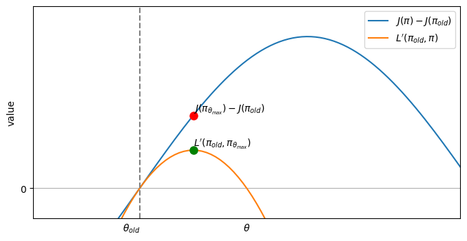
Now, suppose we have found a θ that maximizes L’(π_old, π), then

In other words, the θ that maximizes L’(π_old, π) will ensure monotonic improvement of our real objective - either a strict improvement, or at least staying the same. Moreover, the KL divergence term in L’(π_old, π) can be effectively estimated as well, which means maximizing L’(π_old, π) can be realistically implemented.

The following is pseudo code of this monotonic improvement algorithm:

1: initialize policy parameters θ_0 and value function parameters w_0.
2: for k = 0, 1, 2, … do
3:   collect a sample of episodes D_k by running policy π_k=π(θ_k) in the environment
4:   compute future return g_t for all steps in all episodes
5:   compute advantage estimate A (using any method of advantage estimate) based on the current value function V_k.
6.   get updated policy parameter θ_{k+1} by maximizing L’(π_k, π)
7:   get updated value function parameter w_{k+1} by regressing to g_t on mean-squared error.
8: end for

Compared to A2C, the only difference is in line 6. Instead of taking a small gradient step of J(π_k), it maximizes for a different objective L’(π_old, π). J(π) is a moving target; once the policy moves away from π_k, the gradient derived from J(π_k) is no longer valid, and therefore the algorithm is very sensitive to the choice of step size. L’(π_k, π) is a static anchor. As long as we maximize it, we are guaranteed to move to a better or at least equally good policy, and therefore, the algorithm is very stable.

If this algorithm works in practice, we can probably declare “reinforcement learning is solved”, or at least, “offline batch reinforcement learning is solved”. In reality however, the constant C derived from the theory is so big such that max_π L’(π_old, π) is barely greater than 0. Therefore, the algorithm can only make very small progress in each iteration.

Nonetheless, the theoretical framework has shown what it is achievable and provided a north star and justification for further engineering. TRPO (the predecessor of PPO), two variants of PPO - PPO-clip and PPO-penalty can all be considered engineering optimization to make the theory work in practice, which we will briefly cover in our next section.

Engineering that Makes Theory Work in Practice

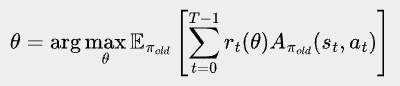
First up we have TRPO, which was introduced by John Schulman et al in 2015. It formulated the problem as maximizing L(π_old, π), while keeping the average KL divergence between π and π_old to be within a hyperparameter 𝛿. More formally, the optimization problem is:

Using second order Taylor expansion, this constraint optimization problem is then approximated by a quadratic optimization problem, which can be solved analytically. TRPO provides excellent stability, but it is considerably slow because it is a second-order optimization algorithm. PPO further simplifies the algorithm by using first order optimization (i.e. stochastic gradient descent).

The 2017 paper by John Schulman et al that introduced PPO included two variants: PPO-penality and PPO-clip.

PPO-penalty adds a KL divergence penalty to L(π_old, π), more specifically:

This is very similar to the formula used in the monotonic improvement algorithm, but instead of using a fixed C derived from theory, it uses a parameter β that gets updated in every round of policy update to control the KL divergence between new and old policy within a certain limit d_tar. More specifically, at the end of each policy update, we calculate the expected KL divergence between π_k+1 and π_k. If the divergence is too much over the target divergence d_tar, we double the penalty β. If it is too much below d_tar, we half β to accelerate the learning.

But PPO-clip is the more popular variant, because of its simplicity and excellent performance in practice. Here is the intuition. When we directly maximize L(π_old, π) without KL penalty or constraint, namely

, gradient updates will keep pushing π(a_t|s_t; θ) towards 1 if A_{π_old}(s_t, a_t) is positive, or pushing towards 0 if A_{π_old}(s_t, a_t) is negative. It causes a big divergence from the old policy, when L(π_old, π) is no longer a good proxy.

PPO-clip prevents such drastic divergence limiting the ratio of π(a_t|s_t; θ) to π(a_t|s_t; θ_old). It puts a ceiling on the ratio if A_{π_old}(s_t, a_t) is positive and a floor on the ratio if A_{π_old}(s_t, a_t) is negative.

More formally, PPO-clip’s objective is:

where

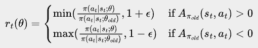
Here, ε is a small positive number between 0 and 1, such as 0.2.

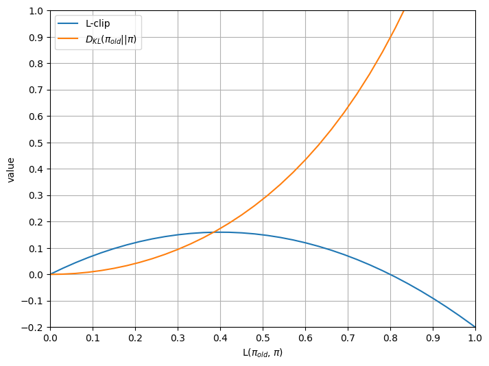
Let’s simulate what happens to r_t(θ) as we maximize PPO-clip’s objective (let’s call it L-clip) when we maximize the unclipped objective L(π_old, π). This way, we can see how clipping helps prevent unbounded change of π that diverges from π_old.

• At the beginning, r_t(θ) won’t be clipped, so L-clip is the same as L(π_old, π). Lots of r_t(θ) are updated in the direction of increasing L-clip, while some of them might move in the opposite direction, but overall L-clip will be increasing, aligning with the trajectory of L(π_old, π).

• As L(π_old, π) continues to increase, more and more r_t(θ) will hit the ceiling or floor and stop contributing to L-clip. L-clip increases significantly slower than L(π_old, π), until some point it stops increasing.

• L(π_old, π) increases more, and now most r_t(θ) having contributed positively to L-clip has been clipped and stopped contributing. Terms that decrease L-clip are now dominating and L-clip decreases as L(π_old, π) increases.

The chart below illustrates the trajectories of L-clip and D_KL(π_old || π) as the unclipped objective L(π_old, π) maximizes.

Trajectories of L-clip and D_KL(π_old || π) as the unclipped objective L(π_old, π) maximizes

Since the introduction of PPO, there are many variants or improvements on top of it, such as GRPO, SPO. All of these algorithms are built on top of the same idea, and I will not go into details of them.

What’s Next?

My original intention for writing this series of blog posts on reinforcement learning was twofold: first, to deepen my own understanding, and second, to show those unfamiliar with the topic that reinforcement learning is not only powerful, but also approachable, and beautiful. But as I write more and more, I am increasingly feeling like I'm writing a story - a story about humanity's endless exploration and overcoming of difficulties; a story about how a group of highly-motivated individuals, standing on the shoulders of each other, pieced together a vast blueprint. I've read many stories like this, but the feeling of writing one myself is completely different.

For those who have developed interests in reinforcement learning through my blog posts and want to keep exploring this fascinating area, you should be aware that I only touched a small part of reinforcement learning - the so-called “model free”, “on-policy”, “batch” reinforcement learning. To develop a big picture and solid foundation in this area, I would definitely recommend Richard Sutton’s book Reinforcement Learning: An Introduction.

I don’t know when I will write the next post for this series; writing this series has been rewarding but also time-consuming. One thing I do know though, is that the story of reinforcement learning has many new chapters to come. It's a continuous, unfolding narrative - a testament to our endless drive to explore and understand - and I can't wait to see what new discoveries are ahead of us.